Introduction
A few weeks ago I went to get some drinks with a few developer friends. We were talking about software at different levels, and one of them talked about how he improved a long running process. This process has two unsorted arrays, and for each item in ArrayA it looks up a value in ArrayB. My friend restructured the algorithm to reduce its time complexity. This led us to a conversation about algorithms, CPU Cycles and Big O Notation.
Big O
Before I talk about the approaches, I have to mention what this “Notation” is. Big O Notation is used to calculate how long an algorithm takes to process N items. Algorithms are classified using this notation to focus on the amount of steps needed to complete, regardless of processing power.
This notation can be used to calculate time complexity or space complexity of an algorithm. Long story short, Big O represents how many items have to be visited (or how many items are in memory) when the algorithm is running.
There is a lot of information on how the Big O Notation works, so I won’t go into details here, the important thing is that as N grows higher, slower algorithms gap gets wider, as seen in the below table:
| N | O(1) | O(Log N) | O(N) | O(N Log N) | O(N2) |
|---|---|---|---|---|---|
| 3 | 1.00 | 1.58 | 3 | 1.43 | 9 |
| 20 | 1.00 | 4.32 | 20 | 26.02 | 400 |
| 300 | 1.00 | 8.23 | 300 | 743.14 | 90000 |
| 5,000 | 1.00 | 12.29 | 5,000 | 18494.85 | 2.50E+07 |
| 100,000 | 1.00 | 16.61 | 100,000 | 5.00E+05 | 1.00E+10 |
I also won’t go into detail on how the Big O notation is calculated for an algorithm, but it is based on loops, inner loops and divide and conquer approaches. A quick example of an algorithm of each category:
- O(1): Look up a value by index or key
- O(Log N): Binary search in a sorted, i.e., keep splitting the array into halves until the value is found
- O(N): Loop through an array
- O(N Log N): A loop within a loop, using divide and conquer, e.g., Quicksort
- O(N2): A loop within another loop, e.g. bubble sort.
Going into code
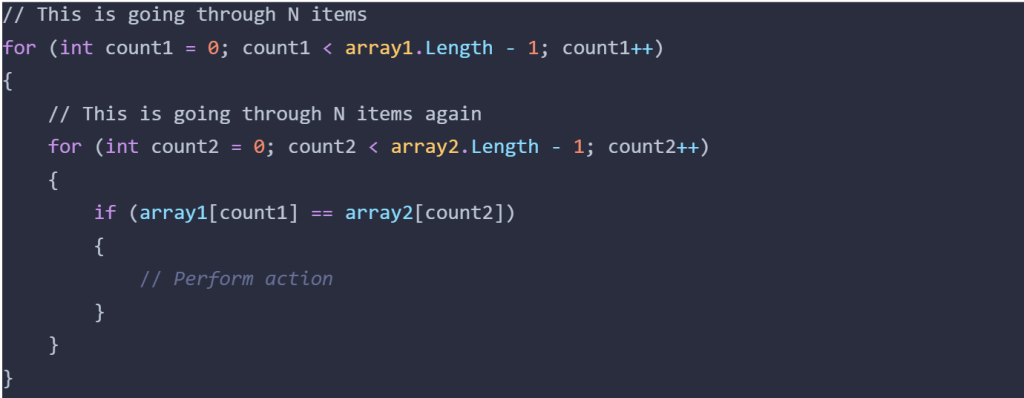
Now onto the code, first is the code in the original state, before any improvements were made. Here we see that, each element in Array1 does a full search on Array2, making the algorithm of N items visit another N items each, this O(N2)

Approach 1: O(N Log N)
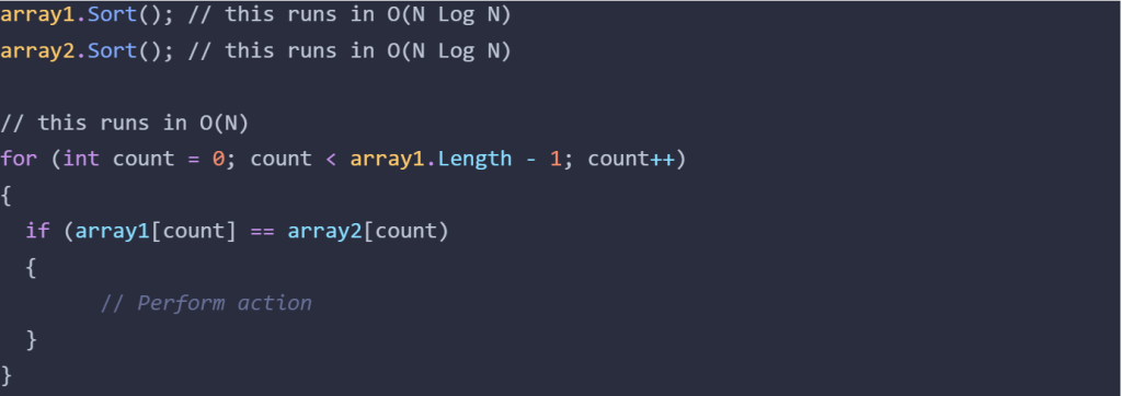
Now we can go into my friend’s solution. Because there are two unsorted arrays, the first step is to sort them, by default this is low to high. Each of these sorts takes O(N Log N), then we have a for loop that cycles through each element once, this part takes O(N). The rules of the notation specify that we use the most complex operation as the complexity, so we can say that the code below runs in O(N Log N).

Approach 2: O(N)
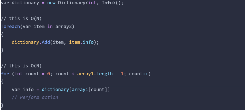
This is the solution that came up in conversation. Instead of sorting both arrays, we can convert Array2 into a Dictionary/HashMap, which loops through each element once, so O(N), then loop over Array1, another O(N) operation.

The theory
From what we know about what Big O represents, we can tell which algorithm is faster just by looking at the code and the loops. Obviously O(N) is faster, we are looping less times over the items of the list. But when we put it to practice we see a different result. I did a quick github repo to test out the algorithms. Here are metrics I gathered by doing all three approaches:
So, what happened here? Why is O(N Log N) faster?
The practice
In practice we see a different result. After running some benchmarks on this repo, we can see that Approach 1 runs faster in actual time. How can that be? Well, since Big O notation only tackles algorithm time complexity, it ignores how the time a CPU takes to look up a value in a Dictionary/HashMap.
We’re talking about CPU cycles now. While in an algorithm each action is a single step, in reality the CPU does more processing in order to do said step. This means that pulling up an item from a Dictionary/HashMap takes up more CPU Cycles that add up.
The Truth
The fact of the matter is that while Approach 1 runs faster in actual time, if we have a large enough data set, Approach 2 will be faster. This can be extrapolated:
With a large enough dataset*, a faster algorithm will run better on a slow CPU, than a slower algorithm in a fast CPU.
* that dataset might be in the trillions.
Conclusion
In the case of my friend’s work, his approach works best because it takes less CPU cycles to pull up an item via index than it does via a key from a Dictionary/HashMap. And this approach will work for millions of items.
But at some point, once we reach a high enough number of items, the algorithm with O(N) will be faster.
Comments
18 responses to “Algorithm vs CPU Cycles”
JILIHOST, simple and straightforward. Don’t expect anything flashy, but it’s easy to use and they seem to have a decent JILI selection. Sometimes less is more, ya know? jilihost
Really insightful article! Thinking about trying online casinos, and the ease of registration at phpgames online casino sounds great – especially with those quick Filipino payment options. A VIP experience is appealing too! 🤔
Phlarologin, easy peasy to log in. No issues there! Sometimes I forget my password, but the reset is quick. Wish there was two-factor authentication for extra security. But hey, all good so far! Go to phlarologin.
It’s fascinating how quickly online gaming evolved in Asia! Seeing platforms like kkk ph link prioritize security & localized payment options (like GCash!) is key to growth. A smart approach to player trust, really.
Bong88999, yeah, it’s alright. Nothing too crazy, but it gets the job done. If you’re looking for something simple and straightforward, it might be your thing. bong88999
Heard about F8betceo. The name’s a bit much, TBH, but the platform is functional. Got some sportsbook options, and some casino games too. Pretty standard stuff, but hey, it works. Try it out if you are curious: f8betceo
Для видеомаркетинга возможно раскрутка в youtube xrumer, но стоит учитывать алгоритмы платформы.
Lifestyle changes are becoming a major topic in modern healthcare systems. People often search how to help liver function through diet, exercise, and supplements. Medical professionals usually stress the importance of personalized guidance.
Video-interactie wordt populairder binnen online communicatie. Sommige platforms gebruiken cam seks xxxbabes4u.com als marketingterm. Gebruiksgemak en duidelijke uitleg verhogen het vertrouwen.
Вітальня часто стає центром усього дому. У публікації ремонт вітальні – стильні рішення https://vseproremont.com/ зібрані актуальні приклади. Вони підкреслюють індивідуальність простору.
Live streams golvar.com.az and live matches online, including the latest football schedule for today. Follow games in real time, find out dates, start times, and key events of football tournaments.
Yolo247site, man, it’s a good place to try your luck. Give it a whirl and see if you strike gold. Click here: yolo247site
Just tried Winjili and I gotta say, not bad! Lots of games to choose from and a decent user experience. Might be your new fav! Check it out winjili
Площадка работает как kraken darknet market с escrow защитой всех транзакций
Після оренди https://cleaninglviv.top/ логічно
ДВС и КПП https://vavtomotor.ru автозапчасти для автомобилей с гарантией и проверенным состоянием. В наличии двигатели и коробки передач для популярных марок, подбор по VIN, быстрая доставка и выгодные цены.
Recommended reading: https://websitedoctor.click/domain/report/124
дизайн проект дома дизайн проект коттеджа